Composing Crossmap Sequences

library(xmap)
library(dplyr)
library(stringr)
library(ggplot2)

PLACEHOLDER: Re-extraction

split_isiccomb <- function(threefour_df) {
  interim <- list()
  interim$isiccomb.rows <-
    threefour_df |>
    filter(str_detect(isiccomb, "[:alpha:]"))
  interim$isiccomb.avg <-
    interim$isiccomb.rows |>
    group_by(country, year, isiccomb) |>
    mutate(value = tidyr::replace_na(value, 0)) |>
    summarise(
      avg.value = mean(value),
      n_isic = n_distinct(isic),
      n_rows = n(),
      .groups = "drop"
    )
  left_join(
    threefour_df,
    interim$isiccomb.avg,
    by = c("country", "year", "isiccomb")
  ) |>
    rename(value.nosplit = value) |>
    mutate(
      value = coalesce(avg.value, value.nosplit),
      split.isiccomb = !is.na(avg.value)
    ) |>
    select(country, year, isic, isiccomb, value, value.nosplit, split.isiccomb)
}

split_links <- indstat$masked_sample |>
  split_isiccomb() |>
  mutate(weights = value / 1000) |>
  tidyr::drop_na(weights)

As in vignette("extract-validate-existing"), we can confirm every country/year group’s links form a valid crossmap with validate_as_xmap():

crossmaps <- split_links |>
  nest_by(country, year, .key = "links") |>
  mutate(
    valid = validate_as_xmap(links, isiccomb, isic, weights),
    xmap = list(as_xmap_tbl(links, isiccomb, isic, weights))
  ) |>
  ungroup()

crossmaps |>
  count(valid)
#> # A tibble: 1 × 2
#>   valid     n
#>   <lgl> <int>
#> 1 TRUE    112

Block-Level Imputation

The crossmaps framework addresses block-level transformation and imputation, whereby instead of modifying rows of data, we treat the collection of code-value pairs for a larger grouping entity as a single observation. For example, the isiccomb code-value pairs in vignette("extract-validate-existing") are parts of the overall aggregate output measure reported for a given country, year. The extracted isiccomb to isic mapping is then a describe how to impute country, year output measures by isic codes from the reported isiccomb observations. The separation of this logic into a standalone object, the crossmap, allows for the imputation to be examined in more granular detail compared to bespoke scripts. This vignette illustrates some of the additional insights that can be derived from analysing crossmaps.

We begin with the collection of extracted country, year isiccomb to isic crossmaps from vignette("extract-validate-existing"). In that vignette, we confirmed that the extracted weights formed valid crossmaps, guaranteeing that the transformations preserved the overall total value. However, this does not provide much insight into how different country, year observations are transformed. In particular, not every country, year observation will be imputed, many observations are already reported directly in isic categories. To understand how much of the larger dataset and which country, year observation blocks require imputation, we can examine properties of the crossmaps directly. To begin, we might look at the distribution of weight types (unit, or fraction) for each country, year:

weight_type <- crossmaps |>
  select(country, year, links) |>
  tidyr::unnest(links) |>
  dplyr::left_join(
    indstat$country_lookup[c("code", "iso3c", "name")],
    by = join_by(country == code)
  ) |>
  rename(country_iso3c = "iso3c") |>
  mutate(weight_type = ifelse(weights == 1, "unit", "frac"))

weight_type |>
  ggplot(aes(x = year, fill = weight_type)) +
  facet_wrap(~country_iso3c) +
  geom_bar(position = "stack") +
  scale_fill_manual(values = c("frac" = "#ef8a62", "unit" = "#67a9cf")) +
  theme_minimal() +
  theme(legend.position = "bottom") +
  labs(y = "`isic` codes", x = "Year", fill = "Weight type")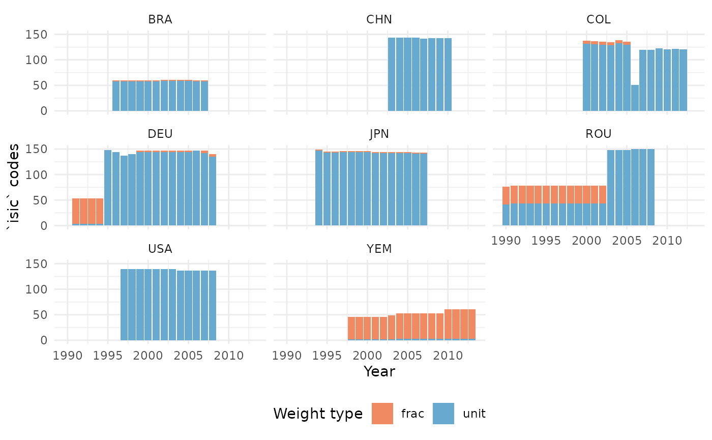

The chart above shows us that for most country, year observations, fractional or splits affect relatively few imputed isic code-value pairs, with most values already directly reported in isic codes. Notice that for most country, years, combined reporting only affects a small number of final isic. Both USA and China (CHN) always reported directly in the isic classification, while Germany (DEU) mostly reported combined isiccomb values over a subset of isic values up from 1991 to 1994 inclusive. 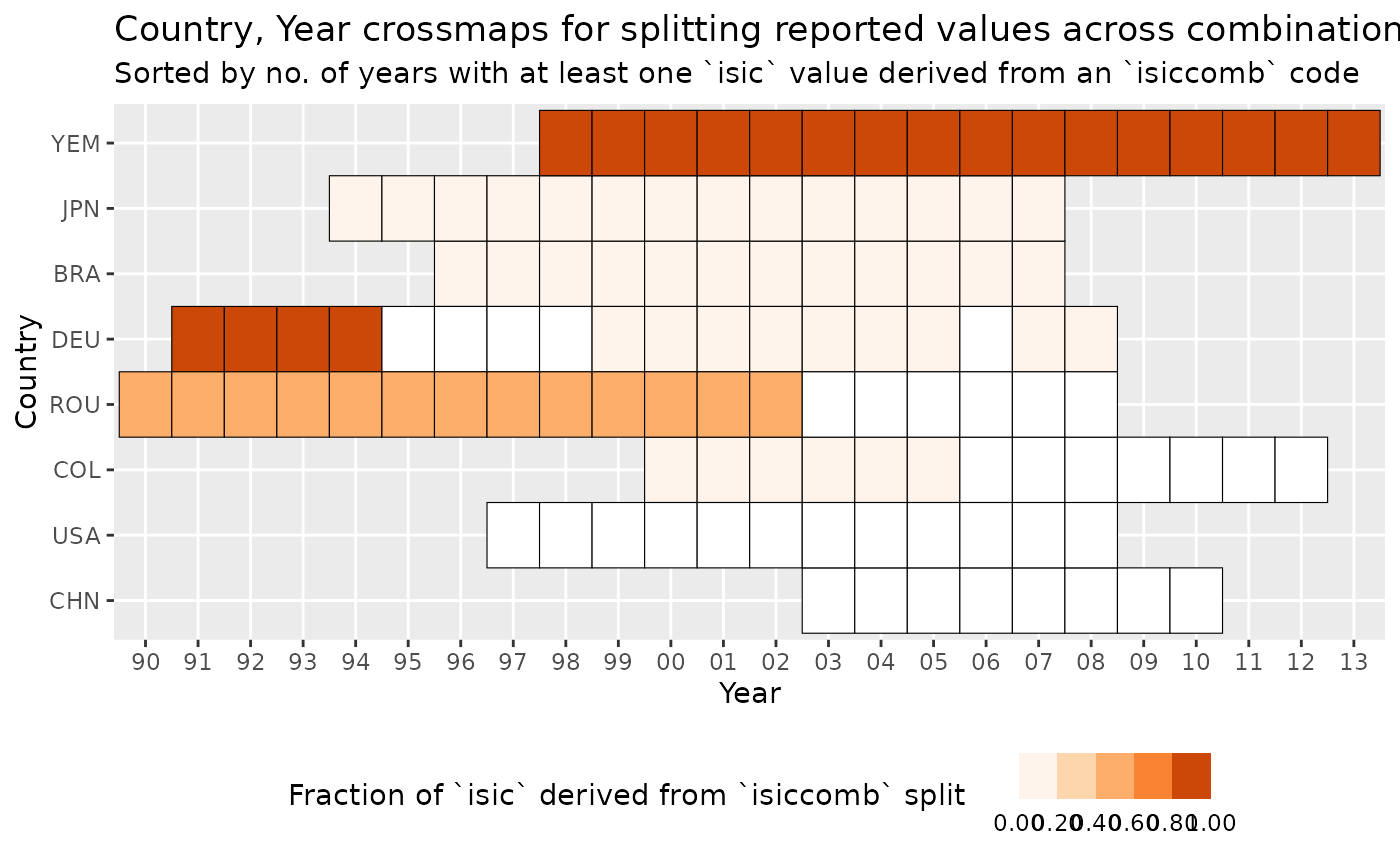Yemen (YEM) is the conspicuous exception, where fractional weights dominate. We can summarise this in a fraction measuring how many isic code-value pairs are derived from splitting isiccomb values:

group_summary <- weight_type |>
  summarise(
    any_isiccomb = any(weight_type == "frac"),
    pct_isiccomb = sum(weight_type == "frac") / n(),
    .by = c(country_iso3c, year)
  ) |>
  mutate(pct_year_isiccomb = sum(any_isiccomb) / n(), .by = c(country_iso3c))

group_summary |>
  ggplot(aes(
    x = as.factor(year),
    fill = pct_isiccomb,
    y = forcats::fct_reorder(country_iso3c, pct_year_isiccomb)
  )) +
  geom_tile(color = "black") +
  ## abbreviate year labels
  scale_x_discrete(labels = ~ str_sub(.x, -2)) +
  scale_fill_stepsn(
    colours = c("white", RColorBrewer::brewer.pal(6, "Oranges")),
    breaks = c(0.0001, seq(0.2, 1, 0.2)),
    limits = c(0, 1),
    labels = scales::label_number(accuracy = 0.01)
  ) +
  # theme_minimal() +
  # move legend to bottom
  theme(legend.position = "bottom") +
  labs(
    x = "Year",
    y = "Country",
    fill = "Fraction of `isic` derived from `isiccomb` split",
    title = "Country, Year crossmaps for splitting reported values across combinations of ISIC Rev. 3 codes",
    subtitle = "Sorted by no. of years with at least one `isic` value derived from an `isiccomb` code"
  )

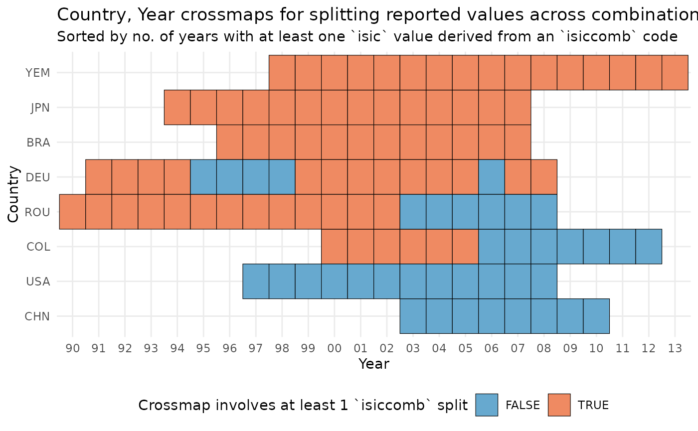
We can also create a binary indicator any_isiccomb for a more coarse-grain overview of which country, year have output values that are redistributed from an actual reported observation under a isiccomb code. This gives an overview of which parts of the harmonised isic dataset have some degree of imputation (orange tiles), and which remain unmodified from the reported values (blue tiles).

group_summary |>
  ggplot(aes(
    x = as.factor(year),
    y = forcats::fct_reorder(country_iso3c, pct_year_isiccomb),
    fill = any_isiccomb
  )) +
  geom_tile(color = "black") +
  scale_x_discrete(labels = ~ str_sub(.x, -2)) +
  scale_fill_manual(values = c("TRUE" = "#ef8a62", "FALSE" = "#67a9cf")) +
  theme_minimal() +
  theme(legend.position = "bottom") +
  labs(
    x = "Year",
    y = "Country",
    fill = "Crossmap involves at least 1 `isiccomb` split",
    title = "Country, Year crossmaps for splitting reported values across combinations of ISIC Rev. 3 codes",
    subtitle = "Sorted by no. of years with at least one `isic` value derived from an `isiccomb` code"
  )

Hierarchical classifcations: Composing to coarser classes

The International Standard Industrial Classification is a strictly hierarchical classification system, whereby each code belongs to one of four nested levels: a 1-letter section, a 2-digit division, a 3-digit group, and a 4-digit class. A class’s first three digits give its group parent, and (since indstat only reports at 3- or 4-digit granularity) isic codes in this dataset are either groups or classes.

Imagine that for analysis purposes we decide on using the 3-digit view of the data. we could easily derive this by calculating the variable isic3 = str_sub(isic, 1, 3) and summarising the 4-digit values within each three digit group with a sum() operation. However, instantiating this aggregation as an explicit crossmap, surfaces some structure in the data that the more efficient aggregation would hide. To illustrate the additional insights we gain, we first create the isic -> isic3 crossmap with as_xmap_tbl(), which also (trivially) validates the links. Unlike isiccomb -> isic – it doesn’t vary by country or year:

(isic3_xmap <- split_links |>
  distinct(isic) |>
  mutate(isic = as.character(isic), isic3 = str_sub(isic, 1, 3), weight = 1) |>
  as_xmap_tbl(from = isic, to = isic3, weight_by = weight))
#> # A crossmap tibble: 151 × 3
#> # with unique keys:  [151] isic -> [61] isic3
#>    .from$isic .to$isic3 .weight_by$weight
#>    <chr>      <chr>                 <dbl>
#>  1 151        151                       1
#>  2 1520       152                       1
#>  3 153        153                       1
#>  4 154        154                       1
#>  5 155        155                       1
#>  6 1600       160                       1
#>  7 171        171                       1
#>  8 172        172                       1
#>  9 1730       173                       1
#> 10 1810       181                       1
#> # ℹ 141 more links

The resulting crossmap isic3_xmap takes 151 isic 3 and 4 digit codes and maps them to 61 isic3 3-digit codes. Given that the target set .to$isic3 is smaller than the source set .from$isic, there must be some aggregation, but how much aggregation is unclear. For example, 1520 is a 4-digit class, but the 0 end digit actually indicates that division 152 is not further decomposed. In ISIC the ending digits 1-9 are used to label legitimate 4-digit sub-classes. This means that the value of 152 is the same as 1520. However, 1520 could be a partial value split from a larger isiccomb code.

To gain an overview of the relationship between ISIC three and four digit classes, we can summarise the crossmap table further using similar summary methods as in the Timor-Leste occupation codes example in vignette("extract-validate-existing"):

(isic3_summary <- isic3_xmap |>
  summarise(
    `.from` = glue::glue_collapse(.from, "+"),
    `n.from` = n(),
    .by = c(.to)
  ) |>
  arrange(desc(n.from)))
#> # A tibble: 61 × 3
#>    .to$isic3 .from                                                        n.from
#>    <chr>     <glue>                                                        <int>
#>  1 292       c("292", "2921", "2922", "2923", "2924", "2925", "2926", "2…      9
#>  2 269       c("269", "2691", "2692", "2693", "2694", "2695", "2696", "2…      8
#>  3 291       c("291", "2911", "2912", "2913", "2914", "2915", "2919")          7
#>  4 154       c("154", "1541", "1542", "1543", "1544", "1549")                  6
#>  5 242       c("242", "2421", "2422", "2423", "2424", "2429")                  6
#>  6 369       c("369", "3691", "3692", "3693", "3694", "3699")                  6
#>  7 151       c("151", "1511", "1512", "1513", "1514")                          5
#>  8 155       c("155", "1551", "1552", "1553", "1554")                          5
#>  9 172       c("172", "1721", "1722", "1723", "1729")                          5
#> 10 202       c("202", "2021", "2022", "2023", "2029")                          5
#> # ℹ 51 more rows

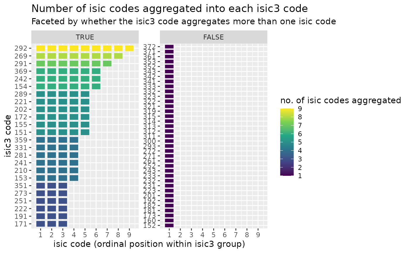
The summary shows that for any given country, year observation with four-digit data, the largest number of four-digit values that could be aggregated is 9 values into the three-digit code 292. A simple facetted heatmap shows the distribution more clearly:

isic3_agg <- isic3_summary |>
  mutate(agg = n.from > 1)

isic3_agg |>
  tidyr::uncount(n.from, .id = "unit", .remove = FALSE) |>
  mutate(agg = forcats::fct_relevel(factor(agg), "TRUE", "FALSE")) |>
  ggplot(aes(
    y = forcats::fct_reorder(.to$isic3, n.from),
    x = unit,
    fill = n.from,
  )) +
  facet_wrap(vars(agg), scales = "free_y") +
  geom_tile(width = 0.8, height = 0.8, color = "white") +
  scale_x_continuous(breaks = scales::breaks_width(1)) +
  scale_fill_viridis_c(breaks = scales::breaks_width(1)) + # + coord_equal()
  labs(
    x = "isic code (ordinal position within isic3 group)",
    y = "isic3 code",
    fill = "no. of isic codes aggregated",
    title = "Number of isic codes aggregated into each isic3 code",
    subtitle = "Faceted by whether the isic3 code aggregates more than one isic code"
  )

Composing crossmap sequences: splitting then aggregating

Although it is useful to be able to summarise and visualise the aggregation step with more granularity and specificity, we also want to be able to obtain the final transformed and imputed country, year observations. Crossmaps are defined on overlapping indexes are composable. For example, if isiccomb->isic and isic->isic3 can be collapsed to isiccomb->isic3 so long as the two isic code sets are identical.

We can use compose_xmap() to check for this overlap, and collapse chains of transformations. This allows us to skip the intermediate calculations and produce isiccomb -> isic3 directly – without ever materialising the intermediate isiccomb-isic-level values:

isiccomb_to_isic3 <- split_links |>
  mutate(isic = as.character(isic), isiccomb = as.character(isiccomb)) |>
  nest_by(country, year, .key = "links") |>
  mutate(
    xmap1 = list(as_xmap_tbl(links, isiccomb, isic, weights)),
    composed = list(tidyr::unpack(
      compose_xmap(xmap1, isic3_xmap),
      everything()
    ))
  ) |>
  reframe(composed)

isiccomb_to_isic3 |>
  filter(country == "276", year == 1991, isiccomb == "151A")
#> # A tibble: 5 × 5
#>   country  year isiccomb isic3 weight_by
#>   <chr>   <dbl> <chr>    <chr>     <dbl>
#> 1 276      1991 151A     151         0.2
#> 2 276      1991 151A     152         0.2
#> 3 276      1991 151A     153         0.2
#> 4 276      1991 151A     154         0.2
#> 5 276      1991 151A     155         0.2

"151A" still lands 1/5 of its weight on each of 151, 152, 153, 154, 155 – 1520’s composed weight rolls straight onto isic3 = 152 – the same picture a two-step split-then-reaggregate would give, just arrived at directly.

Applying the collapsed transformation

apply_xmap() transforms data against a single xmap_tbl, but isiccomb_to_isic3 is a collection of crossmaps – one per country, year. Applying it means nesting the reported isiccomb-level values the same way, then mapping apply_xmap() over each country, year group with its own crossmap:

comb_values <- indstat$masked_sample |>
  mutate(isiccomb = as.character(isiccomb)) |>
  group_by(country, year, isiccomb) |>
  summarise(value = value[!is.na(value)][1], .groups = "drop") |>
  filter(!is.na(value))

direct_isic3 <- comb_values |>
  nest_by(country, year, .key = "values") |>
  mutate(
    xmap_grp = list(
      isiccomb_to_isic3 |>
        filter(.data$country == .env$country, .data$year == .env$year) |>
        as_xmap_tbl(isiccomb, isic3, weight_by)
    ),
    applied = list(apply_xmap(
      values,
      xmap_grp,
      values_from = value,
      keys_from = isiccomb
    ))
  ) |>
  reframe(applied)

direct_isic3
#> # A tibble: 6,375 × 4
#>    country  year isic3 value
#>    <chr>   <dbl> <chr> <dbl>
#>  1 076      1996 151    1000
#>  2 076      1996 152    1000
#>  3 076      1996 153    1000
#>  4 076      1996 154    1000
#>  5 076      1996 155    1000
#>  6 076      1996 160    1000
#>  7 076      1996 171    1000
#>  8 076      1996 172    1000
#>  9 076      1996 173    1000
#> 10 076      1996 181     500
#> # ℹ 6,365 more rows

We can check this against the two-step route: take split_links (which already ran split_isiccomb() to split reported isiccomb values down to isic), derive isic3 = str_sub(isic, 1, 3), and sum value within each country, year, isic3 group by hand. Composing the crossmaps and applying them directly to the original isiccomb-level values should reproduce the same 3-digit totals as this manual split-then-reaggregate:

two_step_isic3 <- split_links |>
  mutate(isic3 = str_sub(as.character(isic), 1, 3)) |>
  group_by(country, year, isic3) |>
  summarise(value_two_step = sum(value, na.rm = TRUE), .groups = "drop")

direct_isic3 |>
  full_join(two_step_isic3, by = c("country", "year", "isic3")) |>
  mutate(diff = value - value_two_step) |>
  summarise(max_abs_diff = max(abs(diff), na.rm = TRUE))
#> # A tibble: 1 × 1
#>   max_abs_diff
#>          <dbl>
#> 1            0

Limitations of composing xmap

Notice that max_abs_diff is not exactly 0 – it’s on the order of 1e-13, far below anything that matters for real data, but not literal floating-point equality either. That residual is a direct symptom of a known limitation of composing weights this way: each composed weight in isiccomb_to_isic3 is a sum of products of the two input crossmaps’ weights, which amplifies floating-point drift relative to either crossmap alone (and would compound further across a longer Reduce()-chained sequence), whereas the two-step route above only ever sums plain values.

Two crossmaps that are each individually valid at the default tolerance can compose into a result that narrowly fails that same tolerance – worth knowing if compose_xmap() aborts on validation with a sequence built from your own data; widening tol on the call is the practical workaround. This is a property of representing weights as plain floating-point numbers, not a bug in the composition itself, and it’s exactly why max_abs_diff above is reported as a small number to eyeball rather than asserted to be identically 0.